ARMA Estimation and Forecasting

[EViews Gareth]

This thread will discuss ARMA estimation and forecasting in EViews – how calculations are performed and how you can mimic those calculations in Excel.

One of the most frequent questions we get regards the difference between AR(1) estimation and lagged endogenous variable estimation. Many people, it would seem, believe that the following two specifications should yield identical results (i.e. should give the same coefficient estimates for both the AR parameter and the constant):

Code: Select all

Y C AR(1) Y C Y(-1)

The confusion arises from the definition of an AR(1) Process. An AR(1) process is simply defined as Yt = c + rYt-1. Given this, is is easy to understand why people believe that estimation of Y with an AR(1) term is the same thing as estimation of Y on a lagged value of Y. However when you are estimating an AR equation, you are not saying that Y follows an AR process, rather you are saying that the error terms follow an AR process. This means that the specification is slightly different:

With some substitution you can re-arrange this specification to become:

or,

Clearly this is different from a regression of Yt on its lagged values:

since the coefficient on the constant is specified differently (although, obviously, you can go from one specification to the other with some simple algebra).

Note that the only difference between the two specifications is the coefficient on the constant. Everything else should remain the same.

[EViews Gareth]

EViews estimates AR processes using a similar substitution to that done above. The linear process:

Becomes:

This is simply a nonlinear least squares problem in the parameters α, β and ρ, which is exactly how EViews estimates the problem.

The follow on question that usually comes after an explanation of how EViews estimates an AR equation, is “how does EViews forecast an AR equation”. It is actually relatively simple, and is based upon the use of the structural residuals,:

Once you have the structural residuals you can create a static forecast, from the equation:

or,


A dynamic forecast is only slightly more complicated:


For the first value of the forecast, you simply use the static value, i.e:


The following EViews program performs static and dynamic forecasts both automatically and manually and shows the results match up:

Code: Select all

rndseed 1 create u 100 series x=nrnd series y=nrnd equation e1.ls y c x ar(1) 'Static Forecast series restemp=y-c(1)-c(2)*x smpl 20 100 e1.fit yhats1 'EViews fitted values (static) series yhats2=c(1)+c(2)*x+c(3)*restemp(-1) 'completely manual calculation 'Dynamic Forecast e1.forecast yhatd1 'EViews forecasted values (dynamic) smpl 20 20 series yhatd2=c(1)+c(2)*x+c(3)*restemp(-1) 'manual calculation of first value smpl 21 100 series yhatd2 = c(1)+c(2)*x+c(3)*(yhatd2(-1)-c(1)-c(2)*x(-1)) 'manual calculation of other values. smpl 20 100 show yhatd1 yhatd2

An Excel file containing the same static and dynamic forecasts can be found here

[EViews Gareth]

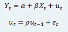
Forecasting an equation with MA terms is a little more tricky. MA(1) estimation is estimation of the following process:


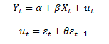
Estimation, and forecasting of MA processes is complicated, especially when backcasting is used to obtain starting observations for the error terms. I’ll leave explanation of backcasting for text books, and concentrate on forecasting an equation without backcasting. The key to a static forecast of an MA process is forecasting the error terms:

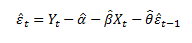
The only problem with this forecast is what value to use for the very first value of the error. With zero backcasting, this is simple, we simply assume that error is zero:


With the error terms forecasted, a static forecast of Y is simply:



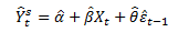
The dynamic forecast of an MA process is even easier. Since the estimate of the error terms is based upon the forecasted value of Y, you can show, easily, that the forecast of the error term becomes zero:


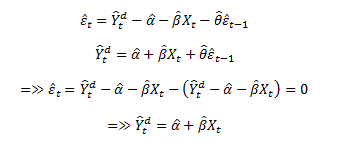
The one exception to this is that, as with the static forecast, the very first error term is calculated as:


The following program shows the manual calculation of the static and dynamic MA forecasts:

Code: Select all

rndseed 1 create u 100 series x=nrnd series y=nrnd equation e1.ls(z) y c x ma(1) 'Static Forecast smpl 1 1 series e=y-c(1)-c(2)*x smpl 2 100 series e=y-c(1)-c(2)*x-c(3)*e(-1) e1.fit yhats1 'EViews fitted values (static) series yhats2=c(1)+c(2)*x+c(3)*e(-1) show yhats1 yhats2 'dynamic Forecast e1.forecast yhatd1 'EViews forecasted values (dynamic) smpl 2 2 series yhatd2 = c(1)+c(2)*x+c(3)*(y(-1)-c(1)-c(2)*x(-1)) smpl 3 100 series yhatd2 = c(1)+c(2)*x smpl @all show yhatd1 yhatd2

An Excel file showing these calculations can be found here

[EViews Gareth]

Here is a very quick example of a static forecast when you have both AR and MA terms:

Code: Select all

rndseed 1 create u 100 series x=nrnd series y=nrnd equation e1.ls(z) y c x ar(1) ma(1) 'Static Forecast series e=0 smpl 2 100 e = y-c(1)-c(2)*X-c(3)*(y(-1)-c(1)-c(2)*x(-1)) - c(4)*e(-1) series yhats2=c(1)+c(2)*x + c(3)*(y(-1)-c(1)-c(2)*x(-1))+ c(4)*e(-1) 'completely manual calculation e1.fit yhats1 'EViews fitted values (static) show yhats1 yhats2